Turn your selfie into a LEGO® brick model
| Philipp GrossUse volumetric regression networks to convert a photo of your face into a 3D voxel model, and then apply stochastic optimization to create LEGO® build layouts.
A few weeks ago, we had the idea to make an app that allows the users to scan an object with their smartphone and convert the photos to a 3D model that can be built with LEGO® bricks. In the following we describe the computer vision and machine learning technologies that were involved in this experiment.
3D reconstruction with volumetric regression networks
Given a series of 2D views of an object as input and mapping it onto a 3D model as output is a classical problem in computer vision also known as Multi View Stereo Reconstruction (MVS). Every solution makes different kinds of assumptions, the most prominent one is scene rigidity, which means that no moving or deforming objects are present within the scene of interest. Other assumptions, which are hard to come by, include the material, intrinsic camera geometry, camera location, camera orientation and light conditions. If these are not known, the problem is ill-posed since multiple combinations can produce exactly the same photographs. In general, the reconstruction requires complex pipelines and solving non-convex optimization-problems.
With the recent advent of deep learning techniques in 3D reconstruction, a promising approach to solving problems like this is to train deep neural networks (DNN). Given a large amount of training data these algorithms have been quite successful in a variety of computer vision applications, including image classification and face detection.
Since 3D reconstruction is in general a difficult problem, we decided to reduce the object category to a category which has been extensively studied before, and which is fun to play with. In 2017 Aaron Jackson et al. published an impressive article 1 where they introduced Volumetric Regression Networks (VRNs) and applied them to face reconstruction. They showed that a CNN can learn directly, in an end-to-end fashion, the mapping from image pixels to the full 3D facial structure geometry (including the non-visible facial parts) with just a single 2D facial image.
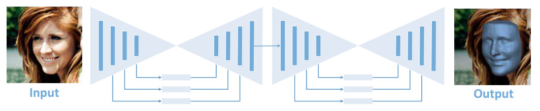 The proposed VRN is a CNN architecture based on two stacked
hourglass networks, which use skip
connections and residual larning. It accepts as input an RGB input of shape
The proposed VRN is a CNN architecture based on two stacked
hourglass networks, which use skip
connections and residual larning. It accepts as input an RGB input of shape
(3, 192, 192) and directly regresses a 3D volume of shape (200, 192, 192).
Each rectangle is a residual module of 256 features. (© Aaron Jackson et al.).
Generously, Jackson et al. also published their code code and a demo based on Torch7. Additionally, Paul Lorenz was so kind to contribute the transfer of the pre-trained VRN model to Keras/Tensorflow with his vrn-torch-to-keras project. This makes loading the model quite simple:
import tensorflow as tf
from tensorflow.core.framework import graph_pb2

def load_model(path, sess):
    with open(path, "rb") as f:
        output_graph_def = graph_pb2.GraphDef()
        output_graph_def.ParseFromString(f.read())
        _ = tf.import_graph_def(output_graph_def, name="")
    x = sess.graph.get_tensor_by_name('input_1:0')
    y = sess.graph.get_tensor_by_name('activation_274/Sigmoid:0')
    return x, y

sess = tf.Session()
model = load_model('vrn-tensorflow.pb', sess)
We load an input image with Pillow and Numpy:
from PIL import Image as pil_image
import numpy as np

def load_image(f):
    img = pil_image.open(f)
    img = img.resize((192, 192), pil_image.NEAREST)
    img = np.asarray(img, dtype=np.float32)
    # The shape is (192, 192, 3), i.e. channels-last order.
    return img
You should only use quadratic images, otherwise the scaling will distort the proportions.
Now, we have everything we need to run the reconstruction:
def reconstruct3d(model, img, sess):
    x, y = model
    # Change order to channels-first
    img = np.transpose(img, (2, 0, 1))

    vol = sess.run(y, feed_dict={x: np.array([img])})[0]
    # vol.shape = (200, 192, 192)

    # Convert image back to original order
    img = np.transpose(img, (1, 2, 0))
    return vol
The output is just a numpy array of dimension 3 where positive values indicate
the voxel position (voxels are the generalization of pixels to the three
dimensional space). You can use
raw2obj.py to
convert it into a colored mesh and write it as a
OBJ-File for further
processing. This simple text file format is understood by various 3D editing
tools and libraries. We use three.js to render it with
WebGL in the browser:
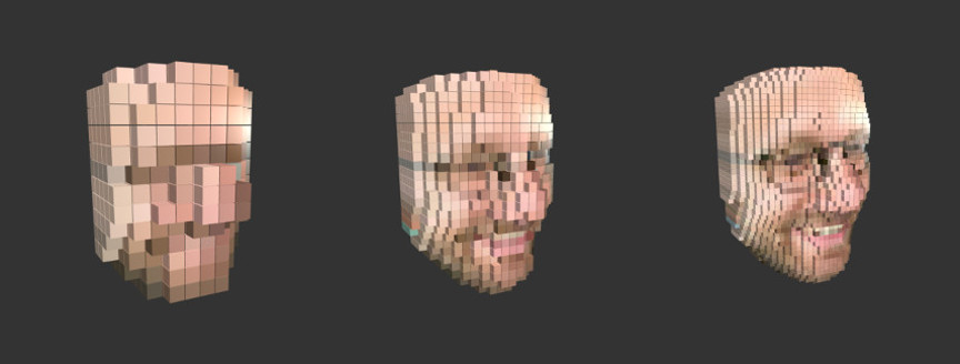
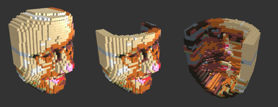
 The input image (left) and rendered output mesh (middle and right).
Obviously, the vrn can't handle glasses, but the results are nevertheless impressive.
Brick model construction
Having a solution to the 3D reconstruction problem at hand it remains to find a LEGO® build layout that approximates the 3D body out of a limited set of pieces. This is also known as legoization or brickification.
The first step is to go back to a voxel representation. If the voxels are mapped onto 1x1 LEGO® bricks, the model doesn't stand in general. So voxels of similar color have to be merged to bigger bricks until a stable structure consisting of one connected component is found. In general, this is a hard combinatorial optimization problem. It was twice openly presented by engineers from the LEGO® company in 1998 and 2001 2, and different solutions were proposed by using stimulated annealing 3, evolutionary algorithms 2, or graph theory 4.
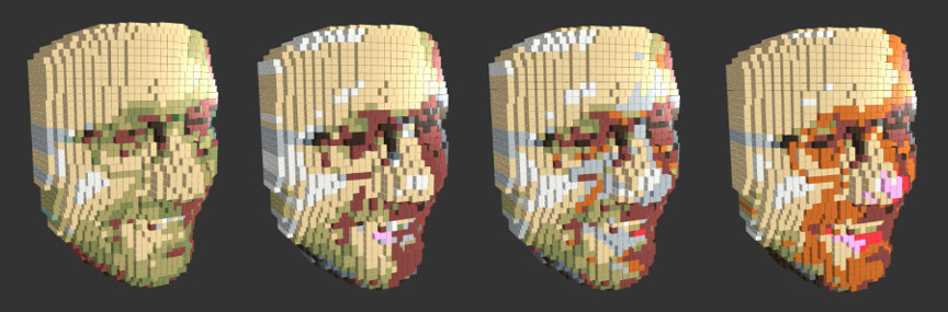
In our case, we are lucky that the shape of the face mesh is just a deformed ball. So, the problem shouldn't be that difficult to solve. First, we rasterize the face mesh with some fixed resolution in order to get voxels:
 Voxels for three different resolutions and counts 563, 3830, 16552 (from left
to right).
Voxels for three different resolutions and counts 563, 3830, 16552 (from left
to right).
Even though the basic bricks are available in many colors at the pick-a-brick LEGO® store, the color space is much smaller than the full RGB space.
 Selection of LEGO® colors (29): Black, Brick Yellow, Bright Blue, Bright
Green, Bright Orange, Bright Purple, Bright Red, Bright Reddish Violet, Bright
Yellow, Bright Yellowish Green, Cool Yellow, Dark Brown, Dark Green, Dark
Orange, Dark Stone Grey, Earth Blue, Earth Green, Flame Yellowish Orange, Light
Purple, Medium Azur, Medium Blue, Medium Lilac, Medium Stone Grey, Olive Green,
Reddish Brown, Sand Green, Sand Yellow, Spring Yellowish Green, White.
Selection of LEGO® colors (29): Black, Brick Yellow, Bright Blue, Bright
Green, Bright Orange, Bright Purple, Bright Red, Bright Reddish Violet, Bright
Yellow, Bright Yellowish Green, Cool Yellow, Dark Brown, Dark Green, Dark
Orange, Dark Stone Grey, Earth Blue, Earth Green, Flame Yellowish Orange, Light
Purple, Medium Azur, Medium Blue, Medium Lilac, Medium Stone Grey, Olive Green,
Reddish Brown, Sand Green, Sand Yellow, Spring Yellowish Green, White.
Since we are interested in building a real-life object instead of just a virtual model, we need to convert the colors with minimal perceptual loss. For that, we map the original colors into the Lab color space and choose the nearest neighbor LEGO® color by using the Delta E 2000 color difference.
 Color mapping to 29 LEGO® colors, by using the L2 metric in RGB space, or
Delta E 76, Delta E 94 and Delta E 2000 color differences in Lab space (from
left to right).
Color mapping to 29 LEGO® colors, by using the L2 metric in RGB space, or
Delta E 76, Delta E 94 and Delta E 2000 color differences in Lab space (from
left to right).
The resulting conversion is not optimal yet, but good enough to keep going.
As we increase the resolution the number of voxels grows cubically which complicates the combinatorial problem and slows down the rendering. Therefore we carve out the inner invisible voxels and just keep a thin shell. Moreover, it suffices to drop the back of the face mesh because the front part already contains the facial geometry.
 Carved voxels with shell size 3. Only the visible voxels are colored.
The upshot of the reduced color palette is that we can merge the 1x1 bricks into larger bricks of the same color which will increase the stability and stiffness of the model. For simplicity, we work only with the basic brick types (1x1, 1x2, 1x3, 1x4, 1x6, 1x8, 2x2, 2x3, 2x4, 2x6, 2x8). As a first naive optimization algorithm, for each layer we merge repeatedly random adjacent bricks if the merged brick is admissable and if all underlying visible voxels have the same color.
Since this algorithm processes each layer independently, it doesn't take into account the overall structure so that some bricks might be disconnected. In order to minimize this effect, for each layer, and each brick we chose to maximize the number of bricks below it connects with, and at the same time minimize the total number of bricks. This gives rise to a cost function that can evaluate any brick layout solution.
Now, we repeat our initial algorithm and replace a solution whenever the cost goes down. This meta-algorithm is also known as random-restart hill climbing. As a final postprocessing step, we compute the connected components of the whole brick layout and remove those that are disconnected from the ground. In most cases this gives an approximate brick layout which seems to be good enough.
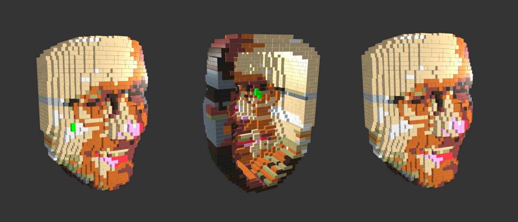 Result after 20 iterations. It has three connected components: A tiny part on
the front marked as green (left), a tiny invisible part (middle) and the main
component (right).
Result after 20 iterations. It has three connected components: A tiny part on
the front marked as green (left), a tiny invisible part (middle) and the main
component (right).
 Primary connected component, rendered with knobs.
Conclusion
Given the fantastic VRN models, it is quite easy to create a LEGO® layout from a single selfie. While the color conversion is far from perfect, it works very well for grayscale pictures or faces that are already close to the LEGO® colors.
Next, we are going to build a real life example and see how well our layout algorithm works in practice!
References
-
Jackson, Aaron S and Bulat, Adrian and Argyriou, Vasileios and Tzimiropoulos, Georgios. Large Pose 3D Face Reconstruction from a Single Image via Direct Volumetric CNN Regression. International Conference on Computer Vision. 2017. ↩
-
Petrovic, Pavel: Solving the LEGO brick layout problem using evolutionary algorithms. Tech. rep., Norwegian University of Science and Technology, 2001. ↩ ↩ 2
-
Gower, Rebecca A H and Heydtmann, Agnes E and Petersen, Henrik G. LEGO: Automated Model Construction. 1998. ↩
-
Testuz, Roman and Schwartzburg, Yuliy and Pauly, Mark. Automatic Generation of Constructable Brick Sculptures. 2013. ↩